
At a glance
Question
I use a CSV file for my data import. I open the CSV file and copy a table out of it into an Excel file.
I have to change the date format and fix the account number, which drops off leading zeros. Is there an easier way to do this?
Answer
Most versions of Excel 2010 and Excel 2013 can use a free add-in from Microsoft called Power Query.
This allows you to directly link to a CSV file and perform data-cleansing procedures while also enabling you to refresh and capture any new data added to the file.
You may need to download the free Power Query add-in from Microsoft. In Excel 2013 and Excel 2016, the Power Query add-in is included in most corporate versions.
Warning: Not all Excel versions in the Office 365 subscription service work with Power Query.
Power Query has many data-cleansing features, but here we will only focus on some features that enable you to easily use a CSV file as a data source.
When you install the add-in into Excel 2010, it is usually available once you open Excel. In Excel 2013, you may need to activate the add-in.
The Power Query add-in is in a different section to most add-ins.
To find it, click the File ribbon tab, then click Options on the left side
On the left side of the Options dialog, click the Add-ins option.
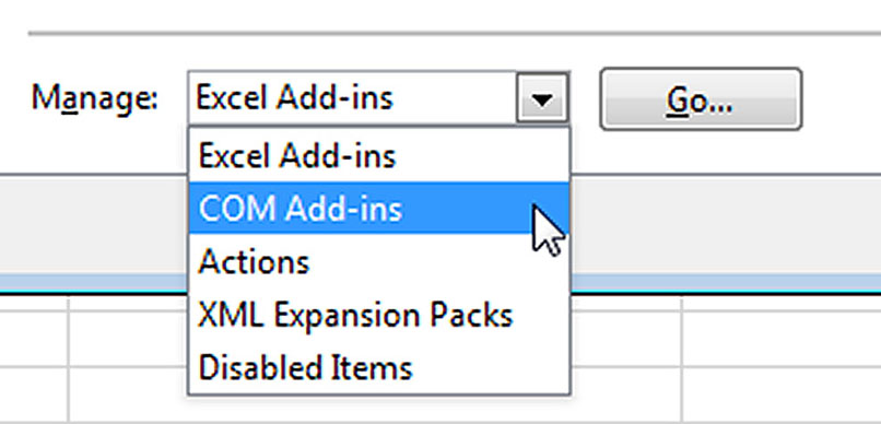
In the Manage drop down at the bottom of the dialog, select COM Add-ins and click the Go button. See Figure 1.
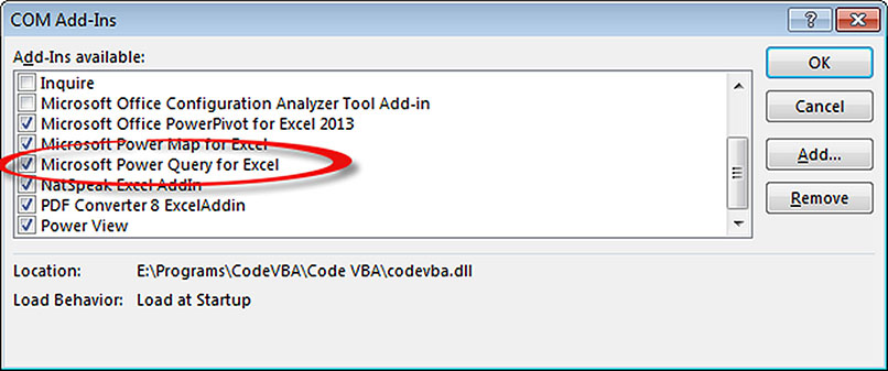
Scroll down the dialog to the Microsoft Power Query for Excel option and tick it. Click OK. See Figure 2.
Once Power Query is installed, it has its own ribbon in Excel 2010 and 2013. It is part of the Data ribbon in Excel 2016.
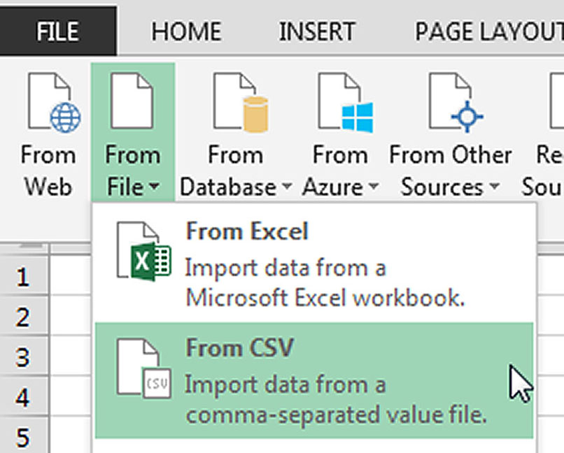
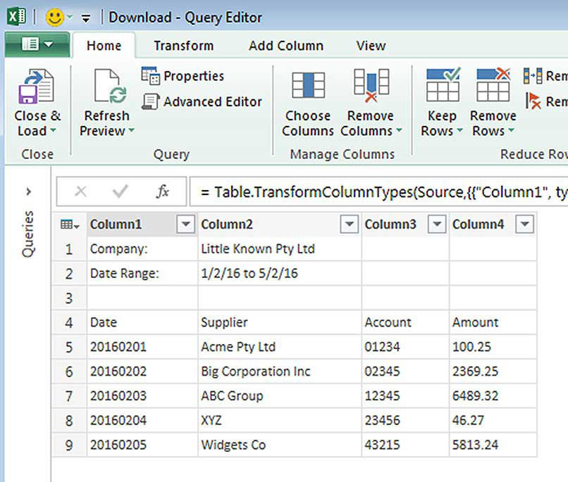
Navigate to the CSV file and click OK. This will open the Power Query window, as per Figure 4.
We will perform three data-cleansing tasks on the file.
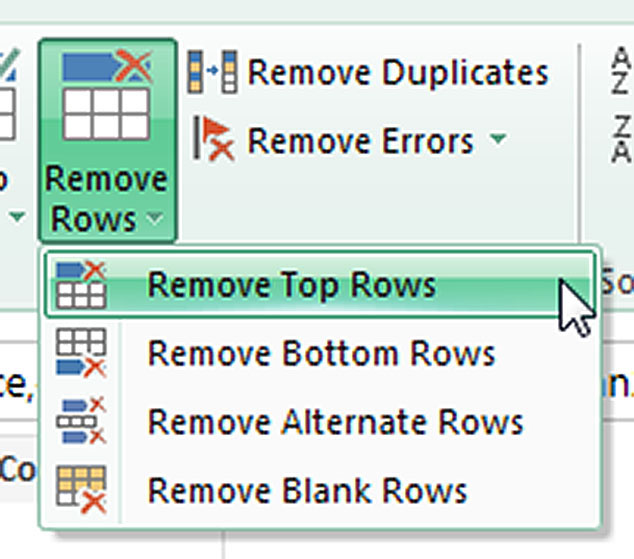
1. Remove the top three rows.
Click the Remove Rows drop down and choose Remove Top Rows, as per Figure 5.
Enter 3 and click OK.
Then click the Use First Row As Headers button. This instructs the Query to treat the first row of the revised layout as column headings.
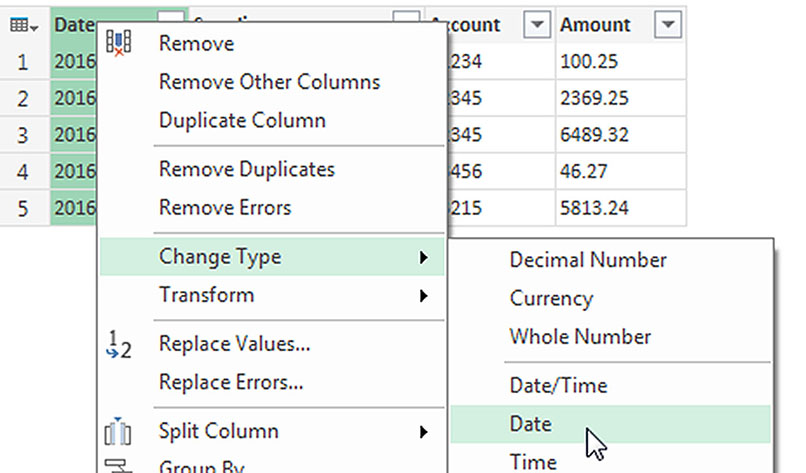
2. Correct the Date column.
Right click the Date column, choose Change Type and then the Date option. See Figure 6.
This has converted a date Excel can’t recognise into one that it can.
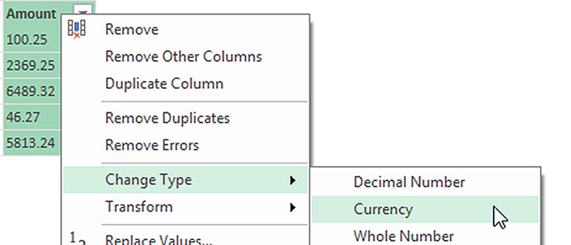
3. Correct the Amount column.
The numbers in the Amount column are left aligned. This usually means they are formatted as text.
Ensure they are imported as values by changing their type.
Right click the Amount column, choose Change Type and choose Currency. See Figure 7.
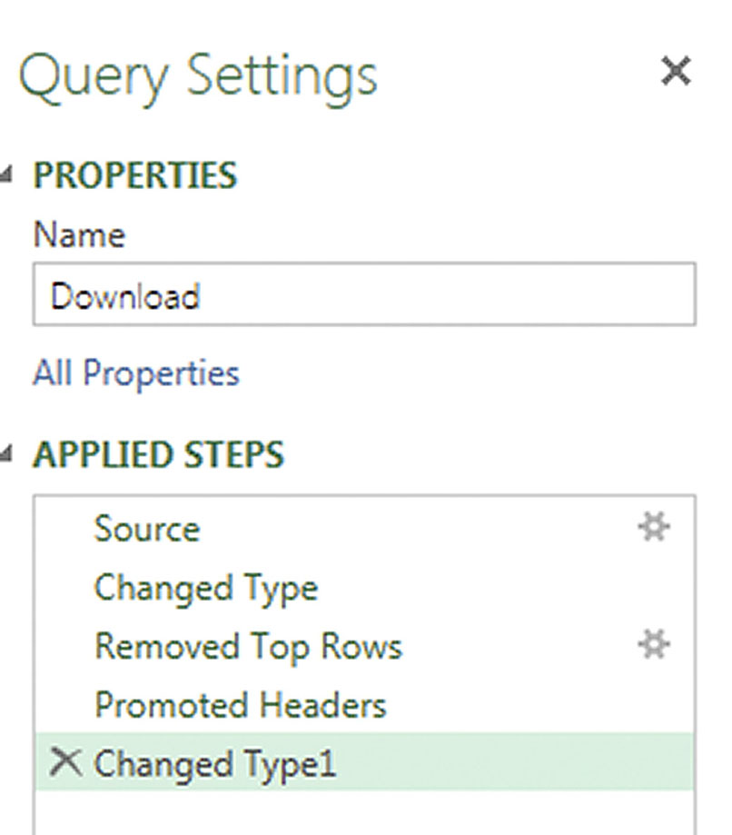
All these changes have been captured in the Query Settings on the right side of the Query window. See Figure 8.
The file name is automatically used as the Query name, but you can change it if you need to.
Even though we changed the type of two columns, it only lists one change.
The Query typically combines column type changes into one step. You can click the small gear icon on the right of an Applied Step to amend the step without having to redo it.
Power Query works a bit like Excel’s Macro Recorder, which captures a sequence of processes.
These Applied Steps will be repeated each time the Excel file is refreshed.
No Undo command
One thing you need to know about the Power Query window is that there is no Undo command.
Typically, if you try something and it doesn’t work, you point to the Applied Step on the right side, delete it and start again.
This returns the data to how it was before the step was applied.
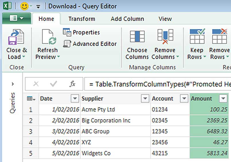
The completed Query window is shown in Figure 9.
To create the table in your file, click the Close & Load icon on the far left side.
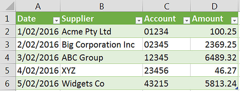
This will create a formatted table of the data from the CSV file in a new sheet. See Figure 10.
This table is ready to use with pivot tables or formula-based reports.
Note the leading zeroes have been retained in the Account column.
When you open a CSV file in Excel, you typically lose any leading zeroes. Power Query avoids that issue.
This technique works well, because to update your data, all you need to do is replace the CSV file with the latest data, being careful to retain its name.
You don’t even need to open the CSV file; you open the Excel file and click Refresh All in the Data ribbon tab and that will automatically update the data, apply the data-cleansing steps and include any extra rows.
Some of Power Query’s other data-cleansing abilities include:
- removing unwanted columns
- filling in blank cells with data from above
- correcting layout issues
- splitting columns
- converting US dates to Australian dates
Power Query works just as well with .txt files and it can import data from most databases.
This has demonstrated the basics of Power Query, but it can also handle large data sets.
In the past, you needed to use formulas or macros to perform these types of data-cleansing exercises, but Power Query makes automating data cleansing much easier.
The companion video and an Excel file may assist your understanding.
Neale Blackwood CPA runs A4 Accounting, providing Excel training, webinars and consulting services to organisations around Australia. Questions can be sent to [email protected]